 Open Exchange
通过 ML 与 IntegratedML 运行一些 Covid-19 ICU 预测(第一部分)
关键字:IRIS, IntegratedML, 机器学习, Covid-19, Kaggle
目的
最近,我注意到一个用于预测 Covid-19 患者是否将转入 ICU 的 Kaggle 数据集。 它是一个包含 1925 条病患记录的电子表格,其中有 231 列生命体征和观察结果,最后一列“ICU”为 1(表示是)或 0(表示否)。 任务是根据已知数据预测患者是否将转入 ICU。
这个数据集看起来是所谓的“传统 ML”任务的一个好例子。数据看上去数量合适,质量也相对合适。它可能更适合在 IntegratedML 演示套件上直接应用,那么,基于普通 ML 管道与可能的 IntegratedML 方法进行快速测试,最简单的方法是什么?
范围
我们将简要地运行一些常规 ML 步骤,如:
- 数据 EDA
- 特征选择
- 模型选择
- 通过网格搜索调整模型参数
与
- 通过 SQL 实现的整合 ML 方法。
它通过 Docker-compose 等方式运行于 AWS Ubuntu 16.04 服务器。
环境
我们将重复使用 integredML-demo-template 的 Docker 环境:
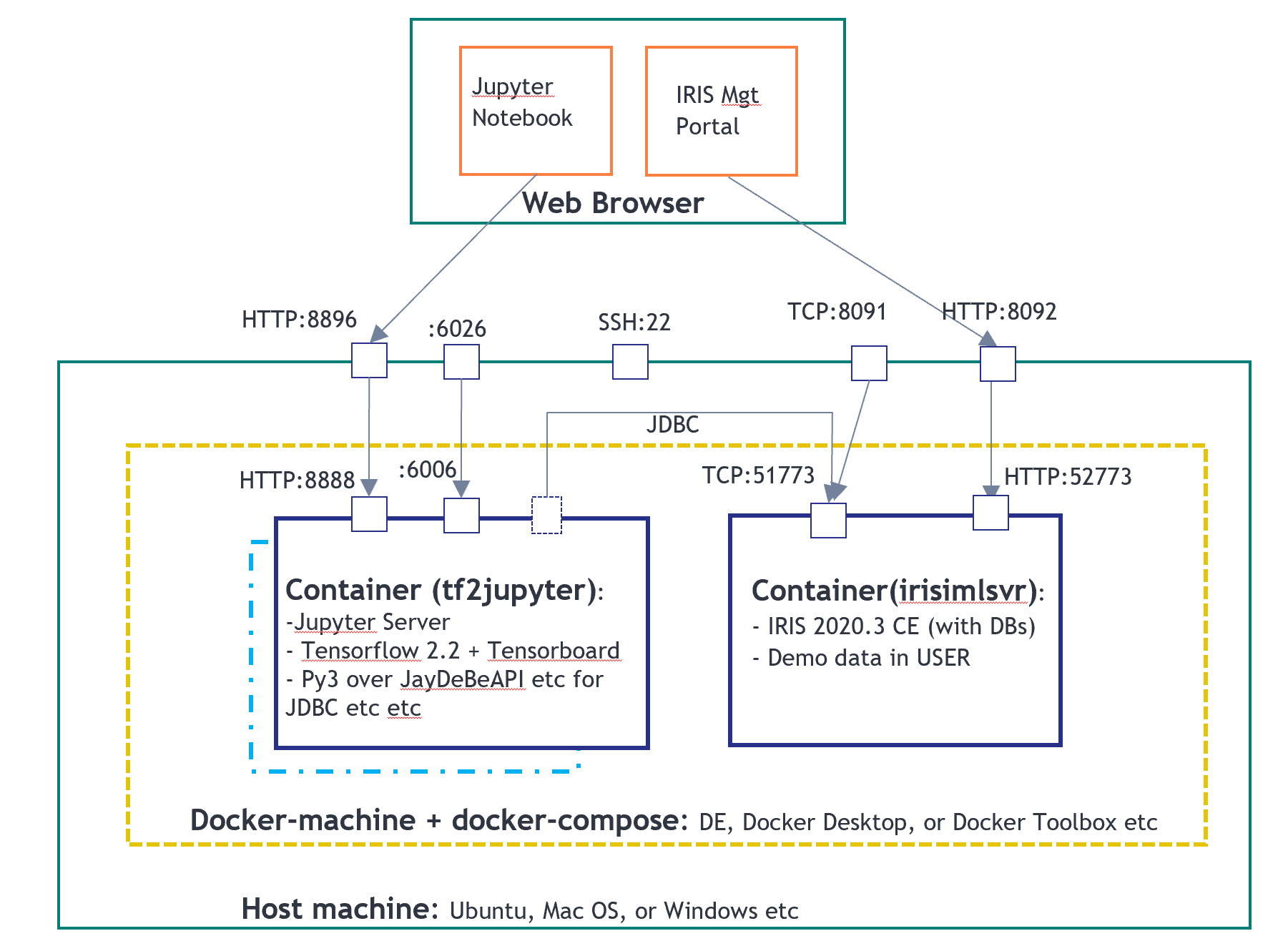
以下 notebook 文件在“tf2jupyter”上运行,带有 IntegratedML 的 IRIS 在“irismlsrv”上运行。 Docker-compose 在 AWS Ubuntu 16.04 上运行。
数据和任务
该数据集包含收集自 385 名患者的 1925 条记录,每名患者正好 5 条记录。 它共有 231 个列,其中有一列“ICU”是我们的训练和预测目标,其他 230 列都以某种方式用作输入。 ICU 具有二进制值 1 或 0。 除了 2 列看上去是分类字符串(在数据框架中显示为“对象”)外,其他所有列都是数值。
import numpy as np
import pandas as pd
from sklearn.impute import SimpleImputer
import matplotlib.pyplot as plt
from sklearn.linear_model import LogisticRegression
from sklearn.model_selection import train_test_split
from sklearn.metrics import classification_report, roc_auc_score, roc_curve
import seaborn as sns
sns.set(style="whitegrid")

import os
for dirname, _, filenames in os.walk('./input'):
    for filename in filenames:
        print(os.path.join(dirname, filename))
./input/datasets_605991_1272346_Kaggle_Sirio_Libanes_ICU_Prediction.xlsx
df = pd.read_excel("./input/datasets_605991_1272346_Kaggle_Sirio_Libanes_ICU_Prediction.xlsx")
df| PATIENT_VISIT_IDENTIFIER | AGE_ABOVE65 | AGE_PERCENTIL | GENDER | DISEASE GROUPING 1 | DISEASE GROUPING 2 | DISEASE GROUPING 3 | DISEASE GROUPING 4 | DISEASE GROUPING 5 | DISEASE GROUPING 6 | ... | TEMPERATURE_DIFF | OXYGEN_SATURATION_DIFF | BLOODPRESSURE_DIASTOLIC_DIFF_REL | BLOODPRESSURE_SISTOLIC_DIFF_REL | HEART_RATE_DIFF_REL | RESPIRATORY_RATE_DIFF_REL | TEMPERATURE_DIFF_REL | OXYGEN_SATURATION_DIFF_REL | WINDOW | ICU | |
|---|---|---|---|---|---|---|---|---|---|---|---|---|---|---|---|---|---|---|---|---|---|
| 1 | 60th | 0.0 | 0.0 | 0.0 | 0.0 | 1.0 | 1.0 | ... | -1.000000 | -1.000000 | -1.000000 | -1.000000 | -1.000000 | -1.000000 | -1.000000 | -1.000000 | 0-2 | ||||
| 1 | 1 | 60th | 0.0 | 0.0 | 0.0 | 0.0 | 1.0 | 1.0 | ... | -1.000000 | -1.000000 | -1.000000 | -1.000000 | -1.000000 | -1.000000 | -1.000000 | -1.000000 | 2-4 | |||
| 2 | 1 | 60th | 0.0 | 0.0 | 0.0 | 0.0 | 1.0 | 1.0 | ... | NaN | NaN | NaN | NaN | NaN | NaN | NaN | NaN | 4-6 | |||
| 3 | 1 | 60th | 0.0 | 0.0 | 0.0 | 0.0 | 1.0 | 1.0 | ... | -1.000000 | -1.000000 | NaN | NaN | NaN | NaN | -1.000000 | -1.000000 | 6-12 | |||
| 4 | 1 | 60th | 0.0 | 0.0 | 0.0 | 0.0 | 1.0 | 1.0 | ... | -0.238095 | -0.818182 | -0.389967 | 0.407558 | -0.230462 | 0.096774 | -0.242282 | -0.814433 | ABOVE_12 | 1 | ||
| ... | ... | ... | ... | ... | ... | ... | ... | ... | ... | ... | ... | ... | ... | ... | ... | ... | ... | ... | ... | ... | ... |
| 1920 | 384 | 50th | 1 | 0.0 | 0.0 | 0.0 | 0.0 | 0.0 | 0.0 | ... | -1.000000 | -1.000000 | -1.000000 | -1.000000 | -1.000000 | -1.000000 | -1.000000 | -1.000000 | 0-2 | ||
| 1921 | 384 | 50th | 1 | 0.0 | 0.0 | 0.0 | 0.0 | 0.0 | 0.0 | ... | -1.000000 | -1.000000 | -1.000000 | -1.000000 | -1.000000 | -1.000000 | -1.000000 | -1.000000 | 2-4 | ||
| 1922 | 384 | 50th | 1 | 0.0 | 0.0 | 0.0 | 0.0 | 0.0 | 0.0 | ... | -1.000000 | -1.000000 | -1.000000 | -1.000000 | -1.000000 | -1.000000 | -1.000000 | -1.000000 | 4-6 | ||
| 1923 | 384 | 50th | 1 | 0.0 | 0.0 | 0.0 | 0.0 | 0.0 | 0.0 | ... | -1.000000 | -1.000000 | -1.000000 | -1.000000 | -1.000000 | -1.000000 | -1.000000 | -1.000000 | 6-12 | ||
| 1924 | 384 | 50th | 1 | 0.0 | 0.0 | 1.0 | 0.0 | 0.0 | 0.0 | ... | -0.547619 | -0.838384 | -0.701863 | -0.585967 | -0.763868 | -0.612903 | -0.551337 | -0.835052 | ABOVE_12 |
1925 行 × 231 列
df.dtypesPATIENT_VISIT_IDENTIFIER int64
AGE_ABOVE65 int64
AGE_PERCENTIL object
GENDER int64
DISEASE GROUPING 1 float64
...
RESPIRATORY_RATE_DIFF_REL float64
TEMPERATURE_DIFF_REL float64
OXYGEN_SATURATION_DIFF_REL float64
WINDOW object
ICU int64
Length: 231, dtype: object当然,设计此问题及其方法有几个选择。 首先,第一个显而易见的选择是,这可以是一个基本的“二元分类”问题。 我们可以将全部 1925 条记录都视为“无状态”个体记录,不管它们是否来自同一患者。 如果我们将 ICU 和其他值都当作数值来处理,这也可以是一个“回归”问题。
当然还有其他可能的方法。 例如,我们可以有一个更深层的视角,即数据集有 385 个不同的短“时间序列”集,每个患者一个。 我们可以将整个数据集分解成 385 个单独的训练集/验证集/测试集,我们是否可以尝试 CNN 或 LSTM 等深度学习模型来捕获每个患者对应的每个集合中隐藏的“症状发展阶段或模式”? 可以的。 这样做的话,我们还可以通过各种方式应用一些数据增强,来丰富测试数据。 但那就是另一个话题了,不在本帖的讨论范围内。
在本帖中,我们将只测试所谓的“传统 ML”方法与 IntegratedML(一种 AutoML)方法的快速运行。
“传统”ML 方法?
与大多数现实案例相比,这是一个相对标准的数据集,除了缺少一些值,所以我们可以跳过特征工程部分,直接使用各个列作为特征。 那么,我们直接进入特征选择。
插补缺失数据
首先,确保所有缺失值都通过简单的插补来填充:
df_cat = df.select_dtypes(include=['object'])
df_numeric = df.select_dtypes(exclude=['object'])
imp = SimpleImputer(missing_values=np.nan, strategy='mean')
idf = pd.DataFrame(imp.fit_transform(df_numeric))
idf.columns = df_numeric.columns
idf.index = df_numeric.index
idf.isnull().sum()
特征选择
我们可以使用数据框架中内置的正态相关函数,来计算每个列的值与 ICU 的相关性。
特征工程 - 相关性
idf.drop(["PATIENT_VISIT_IDENTIFIER"],1)
idf = pd.concat([idf,df_cat ], axis=1)
cor = idf.corr()
cor_target = abs(cor["ICU"])
relevant_features = cor_target[cor_target>0.1]   # correlation above 0.1
print(cor.shape, cor_target.shape, relevant_features.shape)
#relevant_features.index
#relevant_features.index.shape
这将列出 88 个特征,它们与 ICU 目标值的相关度大于 0.1。 这些列可以直接用作我们的模型输入
我还运行了其他几个在传统 ML 任务中常用的“特征选择方法”:
特征选择 - 卡方
from sklearn.feature_selection import SelectKBest
from sklearn.feature_selection import chi2
from sklearn.preprocessing import MinMaxScaler
X_norm = MinMaxScaler().fit_transform(X)
chi_selector = SelectKBest(chi2, k=88)
chi_selector.fit(X_norm, y)
chi_support = chi_selector.get_support()
chi_feature = X.loc[:,chi_support].columns.tolist()
print(str(len(chi_feature)), 'selected features', chi_feature)
88 selected features ['AGE_ABOVE65', 'GENDER', 'DISEASE GROUPING 1', ... ... 'P02_VENOUS_MIN', 'P02_VENOUS_MAX', ... ... RATURE_MAX', 'BLOODPRESSURE_DIASTOLIC_DIFF', ... ... 'TEMPERATURE_DIFF_REL', 'OXYGEN_SATURATION_DIFF_REL']
特征选择 - 皮尔逊相关
def cor_selector(X, y,num_feats): cor_list = [] feature_name = X.columns.tolist() # calculate the correlation with y for each feature for i in X.columns.tolist(): cor = np.corrcoef(X[i], y)[0, 1] cor_list.append(cor) # replace NaN with 0 cor_list = [0 if np.isnan(i) else i for i in cor_list] # feature name cor_feature = X.iloc[:,np.argsort(np.abs(cor_list))[-num_feats:]].columns.tolist() # feature selection? 0 for not select, 1 for select cor_support = [True if i in cor_feature else False for i in feature_name] return cor_support, cor_featurecor_support, cor_feature = cor_selector(X, y, 88) print(str(len(cor_feature)), 'selected features: ', cor_feature)
88 selected features: ['TEMPERATURE_MEAN', 'BLOODPRESSURE_DIASTOLIC_MAX', ... ... 'RESPIRATORY_RATE_DIFF', 'RESPIRATORY_RATE_MAX']
特征选择 - 回归特征消除 (RFE) {#feature-selection---Recursive-Feature-Elimination-(RFE)}
from sklearn.feature_selection import RFE
from sklearn.linear_model import LogisticRegression
rfe_selector = RFE(estimator=LogisticRegression(), n_features_to_select=88, step=100, verbose=5)
rfe_selector.fit(X_norm, y)
rfe_support = rfe_selector.get_support()
rfe_feature = X.loc[:,rfe_support].columns.tolist()
print(str(len(rfe_feature)), 'selected features: ', rfe_feature)
Fitting estimator with 127 features. 88 selected features: ['AGE_ABOVE65', 'GENDER', ... ... 'RESPIRATORY_RATE_DIFF_REL', 'TEMPERATURE_DIFF_REL']
特征选择 - Lasso
ffrom sklearn.feature_selection import SelectFromModel
from sklearn.linear_model import LogisticRegression
from sklearn.preprocessing import MinMaxScaler
X_norm = MinMaxScaler().fit_transform(X)
embeded_lr_selector = SelectFromModel(LogisticRegression(penalty="l2"), max_features=88)
embeded_lr_selector.fit(X_norm, y)
embeded_lr_support = embeded_lr_selector.get_support()
embeded_lr_feature = X.loc[:,embeded_lr_support].columns.tolist()
print(str(len(embeded_lr_feature)), 'selected features', embeded_lr_feature)
65 selected features ['AGE_ABOVE65', 'GENDER', ... ... 'RESPIRATORY_RATE_DIFF_REL', 'TEMPERATURE_DIFF_REL']
特征选择 - RF 基于树:SelectFromModel
from sklearn.feature_selection import SelectFromModel
from sklearn.ensemble import RandomForestClassifier
embeded_rf_selector = SelectFromModel(RandomForestClassifier(n_estimators=100), max_features=227)
embeded_rf_selector.fit(X, y)
embeded_rf_support = embeded_rf_selector.get_support()
embeded_rf_feature = X.loc[:,embeded_rf_support].columns.tolist()
print(str(len(embeded_rf_feature)), 'selected features', embeded_rf_feature)
48 selected features ['AGE_ABOVE65', 'GENDER', ... ... 'TEMPERATURE_DIFF_REL', 'OXYGEN_SATURATION_DIFF_REL']
特征选择 - LightGBM 或 XGBoost
from sklearn.feature_selection import SelectFromModel from lightgbm import LGBMClassifierlgbc=LGBMClassifier(n_estimators=500, learning_rate=0.05, num_leaves=32, colsample_bytree=0.2, reg_alpha=3, reg_lambda=1, min_split_gain=0.01, min_child_weight=40)embeded_lgb_selector = SelectFromModel(lgbc, max_features=128) embeded_lgb_selector.fit(X, y)embeded_lgb_support = embeded_lgb_selector.get_support() embeded_lgb_feature = X.loc[:,embeded_lgb_support].columns.tolist() print(str(len(embeded_lgb_feature)), 'selected features: ', embeded_lgb_feature) embeded_lgb_feature.index
56 selected features: ['AGE_ABOVE65', 'GENDER', 'HTN', ... ... 'TEMPERATURE_DIFF_REL', 'OXYGEN_SATURATION_DIFF_REL']
特征选择 - 全部集成
feature_name = X.columns.tolist() # put all selection together feature_selection_df = pd.DataFrame({'Feature':feature_name, 'Pearson':cor_support, 'Chi-2':chi_support, 'RFE':rfe_support, 'Logistics':embeded_lr_support, 'Random Forest':embeded_rf_support, 'LightGBM':embeded_lgb_support}) # count the selected times for each feature feature_selection_df['Total'] = np.sum(feature_selection_df, axis=1) # display the top 100 num_feats = 227 feature_selection_df = feature_selection_df.sort_values(['Total','Feature'] , ascending=False) feature_selection_df.index = range(1, len(feature_selection_df)+1) feature_selection_df.head(num_feats)df_selected_columns = feature_selection_df.loc[(feature_selection_df['Total'] > 3)] df_selected_columns
我们可以列出通过至少 4 种方法选择的特征:
... ...
我们当然可以选择这 58 个特征。 同时,经验告诉我们,特征选择并不一定总是“民主投票”;更多时候,它可能特定于域问题,特定于数据,有时还特定于我们稍后将采用的 ML 模型或方法。
特征选择 - 第三方工具
有广泛使用的行业工具和 AutoML 工具,例如 DataRobot 可以提供出色的自动特征选择:
从上面的 DataRobot 图表中,我们不难看出,各个 RespiratoryRate 和 BloodPressure 值是与 ICU 转入最相关的特征。
特征选择 - 最终选择
在本例中,我进行了一些快速实验,发现 LightGBM 特征选择的结果实际上更好一点,所以我们只使用这种选择方法。
df_selected_columns = embeded_lgb_feature # better than ensembled selectiondataS = pd.concat([idf[df_selected_columns],idf['ICU'], df_cat['WINDOW']],1) dataS.ICU.value_counts() print(dataS.shape)
(1925, 58)
我们可以看到有 58 个特征被选中;不算太少,也不算太多;对于这个特定的单一目标二元分类问题,看起来是合适的数量。
数据不平衡
plt.figure(figsize=(10,5))
count = sns.countplot(x = "ICU",data=data)
count.set_xticklabels(["Not Admitted","Admitted"])
plt.xlabel("ICU Admission")
plt.ylabel("Patient Count")
plt.show()
这说明数据不平衡,只有 26% 的记录转入了 ICU。 这会影响到结果,因此我们可以考虑常规的数据平衡方法,例如 SMOTE 等。
这里,我们可以尝试其他各种 EDA,以相应了解各种数据分布。
运行基本 LR 训练
Kaggle 网站上有一些不错的快速训练 notebook,我们可以根据自己选择的特征列来快速运行。 让我们从快速运行针对训练管道的 LR 分类器开始:
data2 = pd.concat([idf[df_selected_columns],idf['ICU'], df_cat['WINDOW']],1)
data2.AGE_ABOVE65 = data2.AGE_ABOVE65.astype(int)
data2.ICU = data2.ICU.astype(int)
X2 = data2.drop("ICU",1)
y2 = data2.ICU

from sklearn.preprocessing import LabelEncoder
label_encoder = LabelEncoder()
X2.WINDOW = label_encoder.fit_transform(np.array(X2["WINDOW"].astype(str)).reshape((-1,)))

confusion_matrix2 = pd.crosstab(y2_test, y2_hat, rownames=['Actual'], colnames=['Predicted'])
sns.heatmap(confusion_matrix2, annot=True, fmt = 'g', cmap = 'Reds') print("ORIGINAL")
print(classification_report(y_test, y_hat))
print("AUC = ",roc_auc_score(y_test, y_hat),'\n\n')
print("LABEL ENCODING")
print(classification_report(y2_test, y2_hat))
print("AUC = ",roc_auc_score(y2_test, y2_hat))
y2hat_probs = LR.predict_proba(X2_test)
y2hat_probs = y2hat_probs[:, 1] fpr2, tpr2, _ = roc_curve(y2_test, y2hat_probs) plt.figure(figsize=(10,7))
plt.plot([0, 1], [0, 1], 'k--')
plt.plot(fpr, tpr, label="Base")
plt.plot(fpr2,tpr2,label="Label Encoded")
plt.xlabel('False positive rate')
plt.ylabel('True positive rate')
plt.title('ROC curve')
plt.legend(loc="best")
plt.show()
ORIGINAL
              precision    recall  f1-score   support
           0       0.88      0.94      0.91       171
           1       0.76      0.57      0.65        54
    accuracy                           0.85       225
   macro avg       0.82      0.76      0.78       225
weighted avg       0.85      0.85      0.85       225
AUC =  0.7577972709551657
LABEL ENCODING
              precision    recall  f1-score   support
           0       0.88      0.93      0.90       171
           1       0.73      0.59      0.65        54
    accuracy                           0.85       225
   macro avg       0.80      0.76      0.78       225
weighted avg       0.84      0.85      0.84       225
AUC =  0.7612085769980507
看起来它达到了 76% 的 AUC,准确率为 85%,但转入 ICU 的召回率只有 59% - 似乎有太多假负例。 这当然不理想 - 我们不希望错过患者记录的实际 ICU 风险。 因此,以下所有任务都将集中在如何通过降低 FN 来提高召回率的目标上,希望总体准确度有所平衡。
在前面的部分中,我们提到了不平衡的数据,所以第一本能通常是对测试集进行 Stratify(分层),然后使用 SMOTE 方法使其成为更平衡的数据集。
#stratify the test data, to make sure Train and Test data have the same ratio of 1:0
X3_train,X3_test,y3_train,y3_test = train_test_split(X2,y2,test_size=225/1925,random_state=42, stratify = y2, shuffle = True) <span> </span>
# train and predict
LR.fit(X3_train,y3_train)
y3_hat = LR.predict(X3_test)

#SMOTE the data to make ICU 1:0 a balanced distribution
from imblearn.over_sampling import SMOTE sm = SMOTE(random_state = 42)
X_train_res, y_train_res = sm.fit_sample(X3_train,y3_train.ravel())
LR.fit(X_train_res, y_train_res)
y_res_hat = LR.predict(X3_test)

#draw confusion matrix etc again
confusion_matrix3 = pd.crosstab(y3_test, y_res_hat, rownames=['Actual'], colnames=['Predicted'])
sns.heatmap(confusion_matrix3, annot=True, fmt = 'g', cmap="YlOrBr")
print("LABEL ENCODING + STRATIFY")
print(classification_report(y3_test, y3_hat))
print("AUC = ",roc_auc_score(y3_test, y3_hat),'\n\n')
print("SMOTE")
print(classification_report(y3_test, y_res_hat))
print("AUC = ",roc_auc_score(y3_test, y_res_hat))
y_res_hat_probs = LR.predict_proba(X3_test)
y_res_hat_probs = y_res_hat_probs[:, 1]
fpr_res, tpr_res, _ = roc_curve(y3_test, y_res_hat_probs) plt.figure(figsize=(10,10))

#And plot the ROC curve as before.
LABEL ENCODING + STRATIFY
precision recall f1-score support
0 0.87 0.99 0.92 165
1 0.95 0.58 0.72 60
accuracy 0.88 225
macro avg 0.91 0.79 0.82 225
weighted avg 0.89 0.88 0.87 225
AUC = 0.7856060606060606
SMOTE
precision recall f1-score support
0 0.91 0.88 0.89 165
1 0.69 0.75 0.72 60
accuracy 0.84 225
macro avg 0.80 0.81 0.81 225
weighted avg 0.85 0.84 0.85 225
AUC = 0.8143939393939393
所以对数据进行 STRATIFY 和 SMOT 处理似乎将召回率从 0.59 提高到 0.75,总体准确率为 0.84。
现在,按照传统 ML 的惯例来说,数据处理已大致完成,我们想知道在这种情况下最佳模型是什么;它们是否可以做得更好,我们能否尝试相对全面的比较?
运行各种模型的训练比较:
让我们评估一些常用的 ML 算法,并生成箱形图形式的比较结果仪表板:
# compare algorithms from matplotlib import pyplot from sklearn.model_selection import train_test_split from sklearn.model_selection import cross_val_score from sklearn.model_selection import StratifiedKFold from sklearn.linear_model import LogisticRegression from sklearn.tree import DecisionTreeClassifier from sklearn.neighbors import KNeighborsClassifier from sklearn.discriminant_analysis import LinearDiscriminantAnalysis from sklearn.naive_bayes import GaussianNB from sklearn.svm import SVC #Import Random Forest Model from sklearn.ensemble import RandomForestClassifier from xgboost import XGBClassifier# List Algorithms together models = [] models.append(('LR', &lt;strong>LogisticRegression&lt;/strong>(solver='liblinear', multi_class='ovr'))) models.append(('LDA', LinearDiscriminantAnalysis())) models.append(('KNN', &lt;strong>KNeighborsClassifier&lt;/strong>())) models.append(('CART', &lt;strong>DecisionTreeClassifier&lt;/strong>())) models.append(('NB', &lt;strong>GaussianNB&lt;/strong>())) models.append(('SVM', &lt;strong>SVC&lt;/strong>(gamma='auto'))) models.append(('RF', &lt;strong>RandomForestClassifier&lt;/strong>(n_estimators=100))) models.append(('XGB', &lt;strong>XGBClassifier&lt;/strong>())) #clf = XGBClassifier()# evaluate each model in turn results = [] names = [] for name, model in models: kfold = StratifiedKFold(n_splits=10, random_state=1) cv_results = cross_val_score(model, X_train_res, y_train_res, cv=kfold, scoring='f1') ## accuracy, precision,recall results.append(cv_results) names.append(name) print('%s: %f (%f)' % (name, cv_results.mean(), cv_results.std()))# Compare all model's performance. Question - would like to see a Integrated item on it? pyplot.figure(4, figsize=(12, 8)) pyplot.boxplot(results, labels=names) pyplot.title('Algorithm Comparison') pyplot.show()
LR: 0.805390 (0.021905) LDA: 0.803804 (0.027671) KNN: 0.841824 (0.032945) CART: 0.845596 (0.053828)
NB: 0.622540 (0.060390) SVM: 0.793754 (0.023050) RF: 0.896222 (0.033732) XGB: 0.907529 (0.040693)
上图看起来表明,XGB 分类器和随机森林分类器的 F1 分数好于其他模型。
让我们也比较一下它们在同一组标准化测试数据上的实际测试结果:
import time from pandas import read_csv from sklearn.model_selection import train_test_split from sklearn.metrics import classification_report from sklearn.metrics import confusion_matrix from sklearn.metrics import accuracy_score from sklearn.svm import SVCfor name, model in models: print(name + ':\n\r') start = time.clock() model.fit(X_train_res, y_train_res) print("Train time for ", model, " ", time.clock() - start) predictions = model.predict(X3_test) #(X_validation) # Evaluate predictions print(accuracy_score(y3_test, predictions)) # Y_validation print(confusion_matrix(y3_test, predictions)) print(classification_report(y3_test, predictions))
LR:
Train time for  LogisticRegression(multi_class='ovr', solver='liblinear')   0.02814499999999498
0.8444444444444444
[[145  20]
 [ 15  45]]
              precision    recall  f1-score   support
           0       0.91      0.88      0.89       165
           1       0.69      0.75      0.72        60
    accuracy                           0.84       225
   macro avg       0.80      0.81      0.81       225
weighted avg       0.85      0.84      0.85       225

LDA:
Train time for  LinearDiscriminantAnalysis()   0.2280070000000194
0.8488888888888889
[[147  18]
 [ 16  44]]
              precision    recall  f1-score   support
           0       0.90      0.89      0.90       165
           1       0.71      0.73      0.72        60
    accuracy                           0.85       225
   macro avg       0.81      0.81      0.81       225
weighted avg       0.85      0.85      0.85       225

KNN:
Train time for  KNeighborsClassifier()   0.13023699999999394
0.8355555555555556
[[145  20]
 [ 17  43]]
              precision    recall  f1-score   support
           0       0.90      0.88      0.89       165
           1       0.68      0.72      0.70        60
    accuracy                           0.84       225
   macro avg       0.79      0.80      0.79       225
weighted avg       0.84      0.84      0.84       225

CART:
Train time for  DecisionTreeClassifier()   0.32616000000001577
0.8266666666666667
[[147  18]
 [ 21  39]]
              precision    recall  f1-score   support
           0       0.88      0.89      0.88       165
           1       0.68      0.65      0.67        60
    accuracy                           0.83       225
   macro avg       0.78      0.77      0.77       225
weighted avg       0.82      0.83      0.83       225

NB:
Train time for  GaussianNB()   0.0034229999999979555
0.8355555555555556
[[154  11]
 [ 26  34]]
              precision    recall  f1-score   support
           0       0.86      0.93      0.89       165
           1       0.76      0.57      0.65        60
    accuracy                           0.84       225
   macro avg       0.81      0.75      0.77       225
weighted avg       0.83      0.84      0.83       225

SVM:
Train time for  SVC(gamma='auto')   0.3596520000000112
0.8977777777777778
[[157   8]
 [ 15  45]]
              precision    recall  f1-score   support
           0       0.91      0.95      0.93       165
           1       0.85      0.75      0.80        60
    accuracy                           0.90       225
   macro avg       0.88      0.85      0.86       225
weighted avg       0.90      0.90      0.90       225

RF:
Train time for  RandomForestClassifier()   0.50123099999999
0.9066666666666666
[[158   7]
 [ 14  46]]
              precision    recall  f1-score   support
           0       0.92      0.96      0.94       165
           1       0.87      0.77      0.81        60
    accuracy                           0.91       225
   macro avg       0.89      0.86      0.88       225
weighted avg       0.91      0.91      0.90       225

XGB:
Train time for  XGBClassifier(base_score=0.5, booster='gbtree', colsample_bylevel=1,
              colsample_bynode=1, colsample_bytree=1, gamma=0, gpu_id=-1,
              importance_type='gain', interaction_constraints='',
              learning_rate=0.300000012, max_delta_step=0, max_depth=6,
              min_child_weight=1, missing=nan, monotone_constraints='()',
              n_estimators=100, n_jobs=0, num_parallel_tree=1, random_state=0,
              reg_alpha=0, reg_lambda=1, scale_pos_weight=1, subsample=1,
              tree_method='exact', validate_parameters=1, verbosity=None)   1.649520999999993
0.8844444444444445
[[155  10]
 [ 16  44]]
              precision    recall  f1-score   support
           0       0.91      0.94      0.92       165
           1       0.81      0.73      0.77        60
    accuracy                           0.88       225
   macro avg       0.86      0.84      0.85       225
weighted avg       0.88      0.88      0.88       225
结果显示,RF 实际上好于 XGB。 这意味着 XGB 可能在某种程度上有一点过度拟合。 RFC 结果也比 LR 略有改善。
通过进一步的“通过网格搜索调整参数”运行所选模型
现在假定我们选择了随机森林分类器作为模型。 我们可以对此模型执行进一步的网格搜索,以查看是否可以进一步提高结果的性能。
记住,在这种情况下,我们的目标仍然是优化召回率,这通过最大程度地减少患者可能遇到的 ICU 风险的假负例来实现,所以下面我们将“recall_score”来重新拟合网格搜索。 再次像往常一样使用 10 折交叉验证,因为上面的测试集总是设置为 2915 条记录中的 12% 左右。
from sklearn.model_selection import GridSearchCV # Create the parameter grid based on the results of random search param_grid = {'bootstrap': [True], 'ccp_alpha': [0.0], 'class_weight': [None], 'criterion': ['gini', 'entropy'], 'max_depth': [None], 'max_features': ['auto', 'log2'], 'max_leaf_nodes': [None], 'max_samples': [None], 'min_impurity_decrease': [0.0], 'min_impurity_split': [None], 'min_samples_leaf': [1, 2, 4], 'min_samples_split': [2, 4], 'min_weight_fraction_leaf': [0.0], 'n_estimators': [100, 125], #'n_jobs': [None], 'oob_score': [False], 'random_state': [None], #'verbose': 0, 'warm_start': [False] }#Fine-tune by confusion matrix from sklearn.metrics import roc_curve, precision_recall_curve, auc, make_scorer, recall_score, accuracy_score, precision_score, confusion_matrix scorers = { 'recall_score': make_scorer(recall_score), 'precision_score': make_scorer(precision_score), 'accuracy_score': make_scorer(accuracy_score) }# Create a based model rfc = RandomForestClassifier() # Instantiate the grid search model grid_search = GridSearchCV(estimator = rfc, param_grid = param_grid, scoring=scorers, refit='recall_score', cv = 10, n_jobs = -1, verbose = 2)train_features = X_train_resgrid_search.fit(train_features, train_labels)rf_best_grid = grid_search.best_estimator_rf_best_grid.fit(train_features, train_labels) rf_predictions = rf_best_grid.predict(X3_test) print(accuracy_score(y3_test, rf_predictions)) print(confusion_matrix(y3_test, rf_predictions)) print(classification_report(y3_test, rf_predictions))
0.92
[[ 46  14]
 [  4 161]]
              precision    recall  f1-score   support
           0       0.92      0.77      0.84        60
           1       0.92      0.98      0.95       165
    accuracy                           0.92       225
   macro avg       0.92      0.87      0.89       225
weighted avg       0.92      0.92      0.92       225
结果表明,网格搜索成功地将总体准确度提高了一些,同时保持 FN 不变。
我们同样也绘制 AUC 比较图:
confusion_matrix4 = pd.crosstab(y3_test, rf_predictions, rownames=['Actual'], colnames=['Predicted']) sns.heatmap(confusion_matrix4, annot=True, fmt = 'g', cmap="YlOrBr")print("LABEL ENCODING + STRATIFY") print(classification_report(y3_test, 1-y3_hat)) print("AUC = ",roc_auc_score(y3_test, 1-y3_hat),'\n\n')print("SMOTE") print(classification_report(y3_test, 1-y_res_hat)) print("AUC = ",roc_auc_score(y3_test, 1-y_res_hat), '\n\n')print("SMOTE + LBG Selected Weights + RF Grid Search") print(classification_report(y3_test, rf_predictions)) print("AUC = ",roc_auc_score(y3_test, rf_predictions), '\n\n\n')y_res_hat_probs = LR.predict_proba(X3_test) y_res_hat_probs = y_res_hat_probs[:, 1]predictions_rf_probs = rf_best_grid.predict_proba(X3_test) #(X_validation) predictions_rf_probs = predictions_rf_probs[:, 1]fpr_res, tpr_res, _ = roc_curve(y3_test, 1-y_res_hat_probs) fpr_rf_res, tpr_rf_res, _ = roc_curve(y3_test, predictions_rf_probs)plt.figure(figsize=(10,10)) plt.plot([0, 1], [0, 1], 'k--') plt.plot(fpr, tpr, label="Base") plt.plot(fpr2,tpr2,label="Label Encoded") plt.plot(fpr3,tpr3,label="Stratify") plt.plot(fpr_res,tpr_res,label="SMOTE") plt.plot(fpr_rf_res,tpr_rf_res,label="SMOTE + RF GRID") plt.xlabel('False positive rate') plt.ylabel('True positive rate') plt.title('ROC curve') plt.legend(loc="best") plt.show()
LABEL ENCODING + STRATIFY
              precision    recall  f1-score   support
           0       0.95      0.58      0.72        60
           1       0.87      0.99      0.92       165
    accuracy                           0.88       225
   macro avg       0.91      0.79      0.82       225
weighted avg       0.89      0.88      0.87       225
AUC =  0.7856060606060606

SMOTE
              precision    recall  f1-score   support
           0       0.69      0.75      0.72        60
           1       0.91      0.88      0.89       165
    accuracy                           0.84       225
   macro avg       0.80      0.81      0.81       225
weighted avg       0.85      0.84      0.85       225
AUC =  0.8143939393939394

SMOTE + LBG Selected Weights + RF Grid Search
              precision    recall  f1-score   support
           0       0.92      0.77      0.84        60
           1       0.92      0.98      0.95       165
    accuracy                           0.92       225
   macro avg       0.92      0.87      0.89       225
weighted avg       0.92      0.92      0.92       225
AUC =  0.8712121212121211
结果表明,经过算法比较和进一步的网格搜索后,我们将 AUC 从 78% 提高到 87%,总体准确度为 92%,召回率为 77%。
“传统 ML”方法回顾
那么,这个结果到底如何? 对于使用传统 ML 算法的基本手动处理是可以的。 在 Kaggle 竞争表中表现如何? 好吧,它不会出现在排行榜上。 我通过 DataRobot 当前的 AutoML 服务运行了原始数据集,在对排名前 43 的模型进行比较后,最好的结果是使用模型“具有无人监督学习功能的 XGB 树分类器”实现的相当于大约 90+% 的 AUC(有待使用同类数据进行进一步确认)。 如果真的想在 Kaggle 上具有竞争力,这可能是我们要考虑的底线模型。 我也会将最佳结果与模型的排行列表放在 github 中。 最后,对于特定于医护场所的现实案例,我的感觉是,我们还需要考虑具有一定程度自定义的深度学习方法,正如本贴的“数据和任务”部分所提到的。 当然,在现实情况下,在哪里收集高质量数据列也可能是一个前期问题。
IntegratedML 方法?
上文说明了所谓的传统 ML 流程,其中通常包括数据 EDA、特征工程、特征选择、模型选择和通过网格搜索进行性能优化等。 这是我目前能想到的最简单的适合此任务的方法,我们甚至还没有触及模型部署和服务管理生命周期 - 我们将在下一个帖子中探讨这些方面,研究如何利用 Flask/FastAPI/IRIS,并将这个基本的 ML 模型部署到 Covid-19 X-Ray 演示服务栈中。
现在,IRIS 有了 IntegratedML,它是一个优雅的 SQL 包装器,包装了 AutoML 的强大选项。 在第二部分中,我们可以研究如何以大为简化的流程来完成上述任务,这样我们就不必再为特征选择、模型选择和性能优化等问题而烦恼,同时可获得等效的 ML 结果来实现商业利益。
到这里,如果再塞入使用相同数据快速运行 integratedML 的内容,本帖可能太长了,无法在 10 分钟内读完,因此我将该内容移至第二部分。